Cluster Analysis using K-means Algorithm

In this post, I illustrate the commonly used clustering algorithm called K-means using a self-written Octave functions/codes. Indeed, there are readily available R, python and octave packages/functions which I listed at the end of this post. Cluster analysis groups similar objects together so that objects in the same group are more similar. It can be used for market segmentation, social network analysis, astronomical data analysis, and so on (see for example Bjiuraj etal). K-means clustering is unsupervised learning algorithm that groups a given dataset into k coherent clusters so that each observation belongs to a group with the nearest mean. The number of clusters (Ks) should be known or determined a priori, and for each cluster we need to provide initial means(centroids).

The data used for this post is obtained from the course material of Machine Learning course offered by Prof Andrew Ng from Stanford University.

The steps listed below were followed to implement k-means algorithm:

Step-1: Randomly initialize k points in the dataset as cluster centroid
Step-2: Assign all observations into one of k groups based on which cluster centroid is closest to the observation. The closeness is measured by computing the square of the difference between each observation and the centroids (square of Euclidean distance).
Step-3: Update cluster centroids as the average of the observations inside the k cluster.
Step-4: Repeat steps 2 and 3 until the algorithm converges.

The code in this example is executable in Octave / Matlab Software.

Preparing and Exploring Data

First, import the data

% import the data 
 
		load('ex7data2.mat');

The data has 2 variables and 300 observations. The first five observations are shown below:

N	VAR1	VAR2
1	1.84208	4.60757
2	5.65858	4.79996
3	6.35258	3.29085
4	2.90402	4.61220
5	3.23198	4.93989

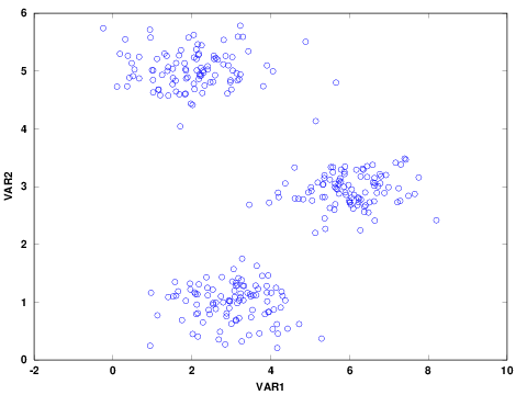
Before analyzing the data, it is good to explore and visualize to have a better sense of the data. For example, check the presence of missing values and visualize the distribution of the data. The summary statistics and scatter plot of the two continuous variables are shown below. There was no missing data in any of the variables. In addition the distribution of the two variables are similar.

Table 1: Summary Statistics

	N	Mean	Std Dev.	Min.	1st Qu.	Median	3rd Qu.	Max.
VAR1	300	3.684	1.926	0.245	2.156	3.232	5.510	8.203
VAR2	300	2.987	1.685	0.206	1.211	2.950	4.808	5.784

Figure 1: Scatter Plot of Variables

Determine Number of Clusters

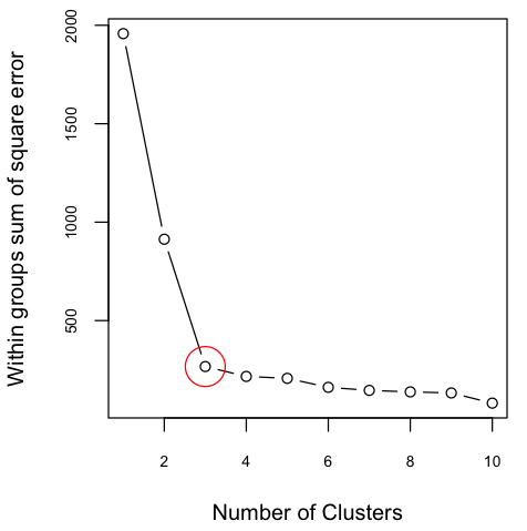
The scatter plot indicates that there are three possible clusters. Often, the number of clusters are not clear or the number of variables are more than two and not straightforward to visualize. In such cases, one approach is to determine the optimal number of clusters using elbow method. The elbow method helps to visualize the sum of square errors (SSE) against the number of clusters, and helps to choose the best number of clusters based on a reasonably minimum SSE achieved for a reasonable small number of clusters. To make this plot, we need to run the algorithm for a number of clusters, for example 1 to 10. To confirm what was seen in the above figure, I plotted SSE against K. The variation on SSE after K=3 is minimal and therefore the figure indicates the presence of 3 clusters.

Figure 2: Sum of Square Error against Number of Clusters

Steps to Implement K-means Cluster

Step-1: Randomly Initialize k Centroids
Three observations are randomly selected from the dataset as initial centroids. Note that the centroids should be unique; however this doesn't guarantee that the k-means can't fall on local optima. Running the algorithm for several different random initials may help to avoid from falling on local optima.


	% K (number of centroids)=3 

	K=3; 

	% X is a two dimensional dataset from which initial centroids are randomly selected  

	rand_idx= randperm(size(X,1));   

	initial_centroids= X(rand_idx(1:K), :); 

	centroids = initial_centroids; 

	previous_centroids = centroids;

Step-2: Assign each observation into one of the centroids
Assign each observation in the dataset to the closest centroid. The function findClosestCentroids, defined below, returns a vector containing the closest centroid for each observation.

 function idx = findClosestCentroids(X, centroids)
  
    [m,n]= size(X); %  m and n are number of rows and columns of the dataset X ;	 

    % Set K		 

    K = size(centroids, 1);		 

    dist= zeros(size(X, 1), K);  	 

    c=0;	 	 

    for i= 1:m		 

		 for k=1:K 	 

            for j= 1:n		 

                % the distance from each observation to a centroid 	 

                c=  c+ (X(i,j)-centroids(k,j)).^2 ;  	 

            end		 

            dist(i,k)= c; %distance of each observation from each centroid 	 

            c=0 ;  % restart c to zero for next iteration  	 

        end	  

    end	  	 

     [min  idx]= min(dist , [], 2);      

      idx; %  a vector containing centroids closest to each observation	   
         
end

Step-3: Update cluster centroids

 % compute new centroids for each cluster using a user-defined function “updateCentroids”. 
 

function centroids = updateCentroids(X, idx, K) 

    clstr=0;	   	

    for k=1:K	  	

    clstr= find(idx==k);  % to find row index where idx==k 	  	

    centroids(k,:)= mean(X(clstr,:));	   

     clstr=0;	   

     end 	      

end

Step-4: Repeat steps 2 and 3 until the algorithm converges.
In this example, the process stops when the maximum number of iteration reached.

 
  % maximum iteration to be 10 		
 
  max_iters = 10;		
 
  K=3;		

% Plot the progress 		

figure;		

hold on;		

% Create palette for coloring 		

palette = hsv(K + 1);		

%-------------------------------		

%Run K-Means algorithm					

%-------------------------------   		

  for i=1:max_iters		

     % Output progress 		

      fflush(stdout); 		

      
      idx = findClosestCentroids(X, centroids); 		


    
      % plot the progress  		

      % Plot simillar clustergroups  with the same color   		

       colors = palette(idx, :); 		

        scatter(X(:,1), X(:,2), 15, colors);	 	


    
      % Plot the centroids as black x's  		

        plot(centroids(:,1), centroids(:,2), 'x', 'MarkerEdgeColor','k', 'MarkerSize', 10, 'LineWidth', 3);	 	


    
      % Plot the history of the centroids with lines	 	

        for j=1:size(centroids,1)	 	

           plot([centroids(j, 1), previous_centroids(j, 1)], [centroids(j, 2), previous_centroids(j, 2)]);	 	

       end	 	


 
     % Title	 		

        title(sprintf('Iteration number %d', i))	 		



         previous_centroids = centroids;	 		

   
     % compute new centroids for each cluster	 		

    
        centroids = updateCentroids(X, idx, K);	 		

         
end;		


    hold off;

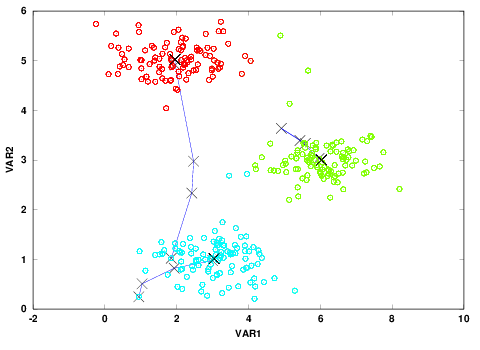
Figure 3: Scatter plot along with three clusters colored in red, green and blue.
The ☓s show the centroids at each iteration for a total number of 10 iterations.

Summary:

I hope this post gives an insight on how k-mean algorithm works. Alternatively, we can use the existing Octave, R or Python functions that can handle K-means cluster analysis. These functions are:

Octave: use the function kmeans from statistics package. For the details, you can refer to Octave documentation

R: use kmeans function from stats package. For the details, you can refer to R documentation.

Python: From scikit-learn package, you can use sklearn.cluster.KMeans class. For the details, you can refer to sklearn.cluster.KMeans documentation.
Or from graphlab package you can use kmeans.create() to perform cluster analysis. For the details, you can refer to graphlab.kmeans.create documentation.